Single layer feedforward neural networks
In this example, we present two implementations of the simplest form of neural networks, the single-layer feedforward neural network. First, we introduce the discrete perceptron classifier, and then the continuous perceptron classifier.
1. Discrete perceptron training
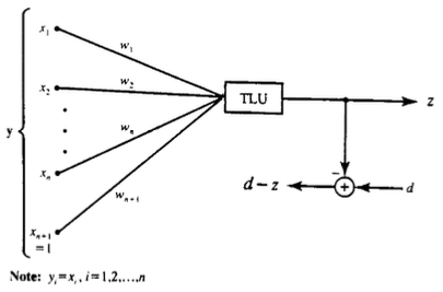
The first classifier is a discrete perceptron, as shown in the figure below. We will use the discrete perceptron learning rule with given values for the learning constant c, initial weights w, and the Threshold Logic Unit (TLU) for the activation function. This example’s main task is to prove that the final weight vector provides the correct classification for the entire training set.
# Import relevant libraries
import numpy as np
import matplotlib.pyplot as plt
# Define inputs and constants
X = np.array([[0.4, 0.8, 0.2, 0.3, 0.2, 1],
              [1, 0.2, 0.5, 0.7, -0.5, 1],
              [-0.1, 0.7, 0.3, 0.3, 0.9, 1],
              [0.2, 0.7, -0.8, 0.9, 0.3, 1],
              [0.1, 0.3, 1.5, 0.9, 1.2, 1]])

X = np.transpose(X)

d = np.array([1, -1, 1, -1, 1])

W = np.array([0.3350, 0.1723, -0.2102,
              0.2528, -0.1133, 0.5012])

c = 2
# Threshold Logic Unit
def TLU(x, T=0):
  if x>=T:
    return 1
  else:
    return -1
# Discrete perceptron training
W = np.array([0.3350, 0.1723, -0.2102,
              0.2528, -0.1133, 0.5012])

pr = []
cr = []
for j in range(10):
  e = 0
  for i in range(5):
    v = np.dot(W, X[:,i])
    z = TLU(v, 0)
    r = d[i]-z
    dW = c*r*X[:,i]
    W += dW

    p = 0.5*(r**2)
    e = e+p
    pr.append(p)
  cr.append(e)
# Pattern Error and Cyle Error Plots
plt.rcParams['figure.figsize'] = [18, 6]
plt.style.use('ggplot')
fig, ax = plt.subplots(1, 2)
ax[0].plot(range(len(pr)), pr,
       linestyle='--',
        color='red')
ax[1].plot(range(len(cr)), cr,
       linestyle='--',
        color='blue')
ax[0].set_ylabel('Pattern Error')
ax[1].set_ylabel('Cycle Error')
ax[0].set_xlabel('Cycle')
ax[1].set_xlabel('Cycle')
fig.suptitle('Pattern and Cycle Error')
plt.show()
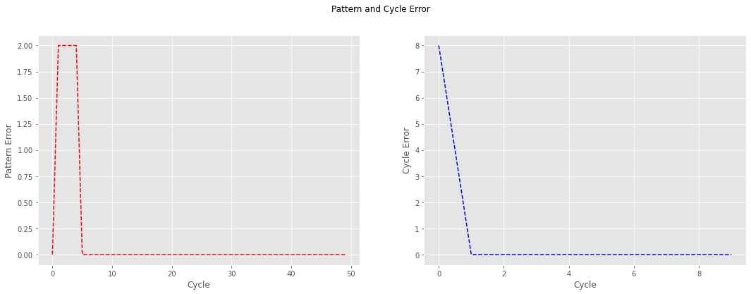
Looking at the pattern and cycle error shown below, one can observe how, after the first cycle, the cycle error converges to zero and remains in that value for the subsequent iterations. When looking at the pattern error, one can observe how the pattern error for the first pattern is zero even before updating the weights; however, that is not the case for the subsequent patterns.
2. Continuous perceptron training
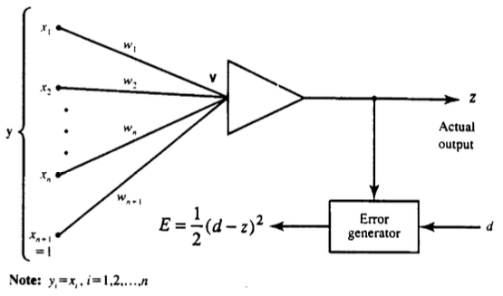
The second example corresponds to a continuous perceptron training as shown in the figure below. The task at hand is to train a perceptron classifier using a logistic activation function $f_1(v) = \frac{1}{1+e^{-v}}$ and the delta learning rule with a learning constant c = 0.2. The parameters x and weights w remain unchanged.
# Define inputs and constants
X = np.array([[0.4, 0.8, 0.2, 0.3, 0.2, 1],
              [1, 0.2, 0.5, 0.7, -0.5, 1],
              [-0.1, 0.7, 0.3, 0.3, 0.9, 1],
              [0.2, 0.7, -0.8, 0.9, 0.3, 1],
              [0.1, 0.3, 1.5, 0.9, 1.2, 1]])

X = np.transpose(X)

d = np.array([1, -1, 1, -1, 1]) # change -1 to zero for sigmoid

W = np.array([0.3350, 0.1723, -0.2102,
              0.2528, -0.1133, 0.5012])

c = 0.2
# Logistic activation function (Sigmoid)
def sigmoid(v):
  return 1 / (1+np.exp(-v))

# First derivative
def dsigmoid(z):
  return z*(1-z)
# Continuos Perceptron Training
W = np.array([0.3350, 0.1723, -0.2102,
              0.2528, -0.1133, 0.5012])

hW = [W] # Used to stored the different weights
cr = []
for j in range(50): # increase the number of cycles for convergence
  e = 0
  for i in range(5):
    v = np.dot(W, X[:, i])
    z = sigmoid(v)
    df2 = dsigmoid(z)
    r = (d[i]-z)*df2
    dW = c*r*X[:,i]
    W += dW
    hW.append(W)
    p = 0.5*((d[i]-z)**2)
    e = e+p
  cr.append(e)
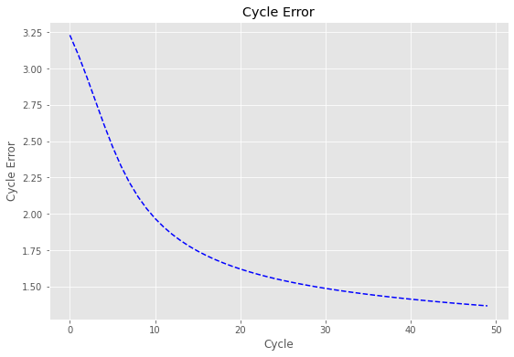
Cycle Error Plot
Looking at the cycle error plot results, one can notice how, unlike the previous approach, the cycle error is not converging to zero as fast as before. One reason for this is that the learning constant c is ten times smaller, causing a slower learning rate. Another outcome that we should expect is that the cycle error will not reach zero even after 1000 cycles; this is because the logistic function used for the activation layer has a lower limit of zero.
# Cyle Error Plot
plt.rcParams['figure.figsize'] = [9, 6]
fig, ax = plt.subplots()
ax.plot(range(len(cr)), cr,
       linestyle='--',
        color='blue')
ax.set_ylabel('Cycle Error')
ax.set_xlabel('Cycle')
ax.set_title('Cycle Error')
Text(0.5, 1.0, 'Cycle Error')